Causal Inference and Machine Learning
This is a blog for my project on the applications of machine learning to discover causal relationships in data in Fall 2022.
How can we use machine learning to uncover causal relationships in the world? Finding causation is a very fundamental question in science. It’s pretty clear to us that when we are young, an increase in our age usually causes an increase in height. But do certain foods cause health benefits or harmful diseases? How can we discover these causal relationships in the data we observe? We normally see machine learning as a tool for training machines to achieve certain (usually predictive or generative) tasks with data. This post exposits how we can possibly leverage recent results showing varying ML performances on data with differing causal structures to discover causal relationships in unknown data.
Every section is dedicated to diving a little bit deeper from the previous one about what the problem we’re looking at is, some current relevant work, and what questions we want to look at next. All the relevant code I write can be found on my github. If you want to learn more about this, reach out to me! I’d love to chat.
What is causal inference and why do I care?
What do we really mean when we say “the economy does better when my favorite political party is in power” or what do we really mean when we say “unvaccinated adults are 3-5 times more likely to get omicron infection”. A very natural property of interest in any dataset is the pattern of correlation - when two events are statistically related. Correlation is an important part of statistics, but what’s more important is how we tend to interpret it. Correlations tell us that two events tend to share some pattern and not that one event is the reason for the other occuring. We really want to say that “the economy is better because of my favorite political party, and not just they happen to occur together. Establishing causal relationships between phenomenon is the study of causal inference. You might have heard the phrase ‘correlation is not the same as causation’. This is true. While it’s true that both the number of tech companies and the number of teddy bears sold has gone up over the last few decades, one does not necessarily cause the other (perhaps both are caused by, among lots of other things, an increase in population sizes leading to more children buying teddy bears and a bigger scientific community built over the years). But this is an example of events that are correlated - they both values have gone up together - but probably not causally related.
I’m interested in causal inference, at the highest level, because it is, in some sense, the most natural question to ask when studying complex datasets. Questions about causation are often the most interesting and, so, inherently the most enlightening in any survey. We know when the economy rises and falls but it’s establishing its cause thats the most interesting. Mathematically, this presents much richer questions: how does one quantitatively establish causation between variables? how is causation structurally different from phenomenon to phenomenon? and how do we quantify that difference? These questions have a lot of implication on not only our understanding of economic and natural phenomenon but also about the human mind and our understanding of how we learn things and form such associations and establish legitimate and unfound causal relationships. I’m interested in these sorts of questions and am looking to explore these in greater depth because I’m fascinated by the question of causation, the mathematical bases on which it can be established, and the understanding of human behavior and learning patterns that this brings.
What question am I interested in?
I’m interested in the interface of causal inference and machine learning (ML). ML refers to the area of computer science and optimization where we train a computer to achieve a certain task using a learning principle and data. The two types of machine learning relevant to this post are supervised learning and semi supervised learning . Supervised learning refers to the method of training algorithms using feature vectors with known labels. Here, the aim is to predict a label y from a feature vector x by training an algorithm on some known features. Semi-supervised learning (SSL) refers to the method of training algorithms with some data with known labels and some with unknown labels. The underlying assumption in most ML problems is that we are trying to find associations or correlations between the labels and features to make predictions; we normally don’t care about their causal structure. It doesn’t seem to matter if x causes y or vice versa since algorithms are expected to perform the same. However, this has shown to not necessarily be true. Scholköpf et al. showed in their 2012 ICML paper that there is in fact a difference in performance in these two cases. SSL algorithms performed better on anticausal problems (i.e. where x causes y ) than in causal problems (vice versa). Figure 1 below illustrates this.
].](/media/ICML_data_hu36da9bb82e926a06828806084ce8066d_113023_419b3a7c6169d24c5817ebd28c4da7d6.png)
Here we see that the performance of SSL on anticausal problems and causal is considerably different to supervised learning. I’m interested in looking at why this is the case and what kinds of problems do better with SSL vs supervised learning.
A toy example where we can see this is in the case of two variables
$$X = N_1$$ $$Y = N_1 + X$$
Where $N_1, N_2 \overset{\mathrm{iid}}{\sim} Be(\frac{1}{2})$. Here there is a clear causal dependency $X \rightarrow Y$.
We can factor the joint probability distribution as
$$P(X,Y) = P(X) P(Y|X) = P(Y) P(X|Y)$$
This factorization is not symmetric since we know that with the current variables, we get the probabilities
$$P(X = x) = 1/2 \text{ for } x=0,1$$ $$P(Y=y) = \begin{cases} \frac{1}{4} & \text{if }y=0,2 \newline \frac{1}{2} & \text{if }y=1\end{cases}$$ $$P(X=x | Y = 0) = \begin{cases} 1 & \text{if }x=0 \newline 0 & \text{if }x=1\end{cases}$$ $$P(Y=y | X = 0) = \begin{cases} \frac{1}{2} & \text{if }y=0 \newline \frac{1}{2} & \text{if }y=1 \newline 0 & \text{if }y=2\end{cases}$$
In ML, we’re usually trying to understand the distribution $ P(Y|X)$ , i.e. given the training data, what is the probability of having any given label. But notice that when we change the distribution of X to, say, $Be(\frac{2}{3})$, then we get the probabilities
$$P(X=x) = \begin{cases} \frac{1}{3} & \text{if }x = 0 \newline \frac{2}{3} & \text{if }x=1\end{cases}$$ $$P(Y=y) = \begin{cases} \frac{1}{4} & \text{if }y=0,2 \newline \frac{1}{2} & \text{if }y=1\end{cases}$$ $$P(X=x | Y = 0) = \begin{cases} 1 & \text{if }x=0 \newline 0 & \text{if }x=1\end{cases}$$ $$P(Y=y | X = 0) = \begin{cases} \frac{1}{3} & \text{if }y=0 \newline \frac{2}{3} & \text{if }y=1 \newline 0 & \text{if }y=2\end{cases}$$
Notice that the distribution for $ P(X|Y)$ does not change but the distribution for $ P(Y|X)$ does. This is a two-variable example to show the assymetry in causal vs anticausal problems and why certain machine learning algorithms might learn $ P(Y|X) $ differently in these cases. The goal for this project is to study this phenomenon. Specifically, I’m interested in the following questions:
-
Can we prove that SSL performs better in anticausal learning problems than other techniques, even for specific cases?
-
Is there an example of a dataset that is traditionally studied with ML techniques agnostic of causal structure that might be better suited to SSL techniques due to an underlying causal structure?
-
Can we actually use these differences in performances to discover causal relationships in data?
Identifiability
To understand this phenomenon better, first, let’s focus on the data and go back to our original motivation: discovering causal structure and finding the causal relationships between different variables. Given features $X$ and labels $Y$, can we distinguish between the causal directions $X \rightarrow Y$ and $Y \rightarrow X$? That is to say, can we ascribe a deterministic mechanism $X \xrightarrow{\varphi} Y$ as apposed to $Y \xrightarrow{\psi} X$ .
A basic assumption that we will make is that each variable is affected by (independent) noise variables $N_Y$ (and $N_X$ for the reverse causal structure). So, the model we will work with is the graph in figure 2.
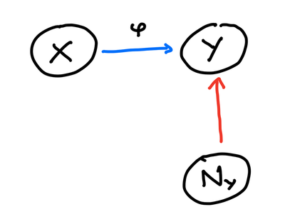
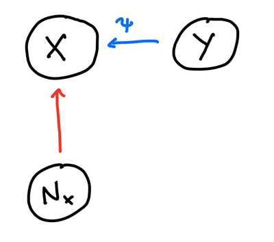
This is a basic structural causal model (SCM) - a model which includes a graph with one vertex per variable, jointly independent noise variables, and a deterministic function for each vertex that depends on the vertex’s parents and noise. This tells us we have a deterministic mechanism $\varphi$ that gives us $Y$ as $Y = \varphi(X, N_Y)$. The question of identifying graphs in causal learning then becomes a question of whether we can ascribe another mechanism from $Y$ to $X$ as shown in figure 3.
It turns out that without any restrictions on the mechanism, the problem of identifying the graph is not feasible. Given variables $X,Y$ along with their probability distribution $P(X,Y)$, you can always fit a mechanism $\varphi$ for either $X \rightarrow Y$ or $Y \rightarrow X$ (the noise variables being understood to be embedded in the graph). This is in the following proposition which states:
Proposition 1. Given two random variables $X$ and $Y$, there is a (measurable) function $f$ and random variable $ N_Y $ such that $Y = f(X, N_Y)$.
Click to see proof
This isn’t the main proof of this section, so I’ll refer you to this paper by Zhang et al. for a nice proof. See Lemma 1.
Without any conditions, the indentification problem is not feasible. This should intuitively feel good - without any assumptions, we have no control over how sensitive the mechanism is to the noise and hence the complexity of $P(Y|X)$.
The question thus becomes: Under what conditions can we only ascribe one causal mechanism between the two variables and not the other (i.e. identify the causal graphs). One possibility is that we make add some structure of the model. So, in our work, we will make the following assumptions. The first will be an assumption about our model and the second will be general SCM assumptions:
-
The mechanism is an Additive Noise Model (ANM), i.e. $$\varphi (X, N_Y) = \phi(X) + N_Y$$ for some function $\phi$, where $N_Y$ and $X$ are independent.
-
The usual assumptions of SCMs also hold: the independence of the mechanism and input ( $P(Y | X)$ and $X$ ), Markov compatibility ( $P(Y)$ just depends on it’s parent $X$ - which is trivial in our case ), and causal sufficiency.
The first assumption is our main one. Hoyer et al. showed in their 2009 NeurIPS paper that under the ANM assumption, we can recover the causal mechanism in most cases. Before we state the main theorem, it is worth noting that since $X$ and $N_Y$ are independent, the joint distribution $ P(X,Y) $ can be rewritten as
$$ P(X = x, Y = y) = P(X = x, N_y = y - \phi(x))$$ $$= P_{X}(X = x) \cdot P_{N_Y}(N_Y = y - \phi(x)) $$
This equivalent restatement will make the theorem easier to state:
Theorem 1. Given $ X, N_Y$ , and $Y$ that satisfy an ANM with a function $ \phi$, if there is a backward mechanism of the same form, then $\phi, P_X, P_{N_Y}$ must satisfy the following differential equation:
$$\xi''' = \xi'' \left( -\frac{\nu''' \phi'}{\nu''} + \frac{\phi''}{\phi'} \right) - 2 \nu '' \phi'' \phi' + \nu' \phi''' + \frac{\nu' \nu''' \phi'' \phi'}{\nu''} - \frac{\nu' (\phi'')^2}{\phi'}$$
where $\nu := \operatorname{log} P_{N_Y}$ and $\xi := \operatorname{log}P_X$, and we also have that $\nu''(y-\phi(x))\phi'(x) \neq 0$ .
Also, we have that if these conditions hold, then if there is a $y$ for which $\nu''(y-\phi(x))\phi'(x) \neq 0$ is true for every $ x $ aside from a countable set, then the set of all $ P_X $ which admit a backward model is 3-dimensional (i.e. can be contained in a 3-dimensional affine space).
Of course, here we are assuming that all the relevant functions are thrice differentiable.
Click here if you’re interested in the proof
You can find my write up and notes on the proof here. The general idea of the proof is that just as we can factor the joint distribution $P_{X,Y}$ into a product of distributions $P_X \cdot P_{N_Y}$ , if a backword model exists, we could similarly factor it into $P_Y \cdot P_{N_X}$ . Taking second order partial derivatives of (the logs of) both of these factorizations give different expressions which we set to be equal since they’re the derivatives of the same distribution. Setting the derivatives equal and rearranging terms gives us part one. Part two follows from the theory of linear differential equations.
The differential equation seems quite arbitrary, but let’s understand at a high level what this tells us. The differential equation is of order 3 (since the highest derivative taken is a third derivative). We can also see that it is linear in $\xi$ ; that is, it can be written as
$$a_0 + a_2 \xi'' + a_3 \xi ''' = b(x,y)$$
and the solution space must be 3-dimensional (see proof for details). Given that the dimension of the space of every possible solution $\xi$ is infinite dimensional, this tells us that almost every ANM $\varphi$ does not admit a backwards model since most $ \phi, P_X, P_{N_Y} $ don’t satisfy the above differential equation.
On a side note, a fun corollary of this theorem is that if $ \xi''' = \nu''' = 0$ everywhere, then the only $\phi$ for which a backward model exists is for linear $\phi$ . This tells us that, for example, in the case where $ P_X$ and $P_{N_Y}$ are Gaussian, only linear $\phi$ admit backward models.
Click here if you’re interested in the proof
This proof follows pretty much exactly as in the Hoyer paper, but if you’d like to see it, you can find my write up and notes here
What this tells us about the identification problem is that if given variables $X,Y$ , if we can fit an ANM $\varphi : X \rightarrow Y$ , then with probability 1, we can assume that the causal relationship is $X \rightarrow Y$ . In the next section, we’ll include some experiments to show how we can use this theoretical results in some practical cases with both with real data and synthetic examples. Then, we’ll move to studying the SSL problem under these conditions.
For some further reading for anyone interested, Zhang and Hyvärinen showed in their 2010 AUI paper similar results for postlinear ANM models, which apply a further nonlinear transformation to the ANM we used. The proof techniques used there are quite similar to the proof technique used here!
Experiments
So how do we put this into practice? We’ll work through this by working backwards. What we saw was that if we can fit an ANM to data $X,Y$ , then we can say with probability one that the correct causal relationship is $ X \rightarrow Y $ , unless, of course, the model is linear in $Y$ , which is the corollary mentioned after theorem 1. Here is the gameplan:
Step 1: We’ll set up our data X and Y assuming they are not statistically independent. Of course, in practice, we would need to test this, but for the sake of explanation here, we will assume this.
Step 2: We’ll then perform a regression of $Y$ onto $X$ . More specifically, we’ll split the data first into training data for our model and testing data; so really, training a regression model to regress $Y_{\text{train}}$ onto $X_{\text{train}}$ and then make our predictions on the testing set $\hat{\phi} (X_{\text{test}})$ .
Step 3: We’ll finally compute the estimates of the residuals $\hat{N} = Y_{\text{test}} - \hat{\phi} (X_{\text{test}})$ .
Step 4: Then, we test whether $\hat{N}$ is statistically independent from $X_{\text{test}}$ . If it is, then the model $Y = \phi(X) + N_X$ is consistent with the data and we accept the ANM otherwise we reject it.
Step 5: To see if we have a backward model as well, we’ll do the same the same process to see if the model $X = \psi(Y) + N_Y$ is consistent with the data. If so, we’ll accept the reverse model; if not, we reject it.
Once we do this, if neither model is accepted, then we failed to fit an ANM either way and we can’t make any causal inferences from the experiment. If one model is accepted and the other rejected, we have evidence to support the respective causal direction - forward or reverse. If both models are accepted, then either causal direction is valid.
A couple of technical details: the regression that I am going to use is sklearn’s Support Vector Regression (SVR). One can use more advanced regression methods, but I found that this is sufficient for our purposes. To test independence, I will be using the HSIC from the work of Gretton et al. in their 2007 NeurIPS Paper - a test that is now very standard in applications. All code can be found on my github.
Experiment 1 - Synthetic Data
In our first experiment, we’ll recreate some of Hoyer et al’s results and use synthetic data - a good place to start with these sorts of experiments.
We sample $X$ and $N$ from a standard normal Gaussian distribution and take their absolute values to the power $q$ - a parameter to measure how Gaussian the distributions are. $q=1$ gives us a usual Gaussian distribution; $q>1$ gives us a super-Gaussian distribution; $q<1$ gives us a sub-Gaussian distribution. We’ll then take $Y = X + bX^3 + N$ where $b$ is a parameter that controls the amount of linearity. Notice that $$b = 0 \implies Y = X + N$$ and so $Y$ is linear in that case.
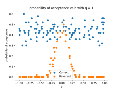
For $q=1$ , we take 100 values of $b$ between $-1$ and $1$ and took the average of 50 experiments in each case. Figure 4 shows the probability of the forward and reverse models being accepted. As we would expect, the probability of the reverse model being accepted is significant only around $b=0$ where the model is linear and essentially $ 0 $ otherwise, whereas the forward (correct) model is usually accepted.
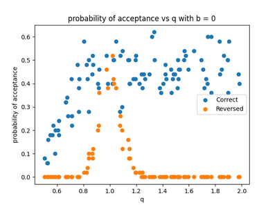
For $b=0$ , i.e. the linear case, we similarly take 100 values of $q$ between $ 0.5 $ and $ 2 $ and plot the average of 50 experiments per value of $q$ in figure 5. The reverse model is accepted around $ q=1 $ as seen before and rejected for the super-Gaussian and sub-Gaussian cases. So the model can solve the linear sub-Gaussian and super-Gaussian cases.
Experiment 2 - Real Data
“Great! We can find causal relationships in data where we build those relationships in. Now what?”
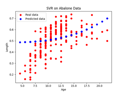
I’m glad you asked! Let’s shift our focus to a real dataset. For the purposes of illustration the method in practice, we’ll use the UCI abalone dataset. Abalone are snails and it’s tricky to determine their age. To do this, one needs to cut the shell through the cone, stain it, and count the number of rings through a microscope. The number of rings is closely related to its age and gives us our best estimate, but, as UCI puts it, “[it’s a] boring and time consuming task.” A standard machine learning problem is to use easier to obtain measurements, such as the length of its shell among other things, to predict its age. Our feature, $X$ is the length of the shell and the label we want to predict, $Y$ is its age. This is a fine task, but in the spirit of causal learning, let’s ask instead: what is the causal relationship between $X$ and $Y$ ? Does age cause the length of the shell or does the length cause age? Here, it’s obvious that it’s the former - we expect that length causes age. This is good, because we can use our theory to verify this hypothesis.
After running the same experiments as in experiment 1, we get the following regressions and residuals.
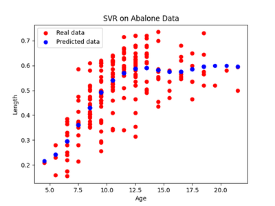
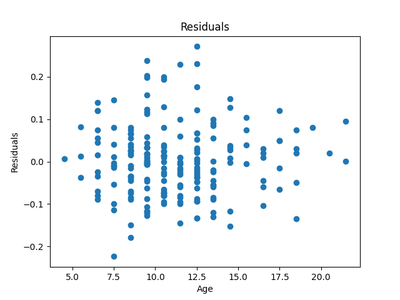
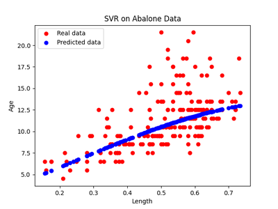
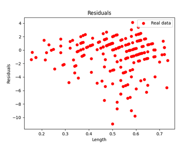
The HSIC score for the testing data for the forward model $X \rightarrow Y$ was $0.6$ with the threshold being $ 0.3$ . So the forward model was rejected. The HSIC score for the reverse model $Y \rightarrow X$ was $ 0.2 $ with a similar threshold and so the reverse model was accepted. Thus we have seen that this is a case of anticausal learning and, in fact, it’s the age of the snail that causes the length of the shell and not the other way around.
These are simple examples that serve as evidence to the interesting claim that one can use machine learning techniques to find causal relationships in data.
More complex examples and what can go wrong
Where do we go from here. A first question one might have is that does this method work for more than two variables? Well, yes - but with a caveat.
The key experiment here involves some synthetic data again. We start by defining the following random variables
$$W \sim Unif(-5,5)$$ $$ X = \frac{W^3}{10} + N_X$$ $$ Y = \cos(W) + N_Y$$ $$ Z = \ln{\sqrt{|X|+1}} + \cos(Y) + N_Z$$
where $N_X, N_Y, N_Z \overset{\mathrm{iid}}{\sim} Unif(-1,1)$ . Clearly, the DAG that we’re working with is the following one in figure 10.
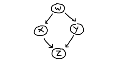
Using the exact same method as in experiment 1, we run through every possible combination of causal directions between each pair of variables (cycling through each dag) and we get that the correct causal graph is accepted 78% of the time (in 1000 random experiments) while the incorrect ones are rejected. The problem with this method in real applications, however, is that as the number of variables $ n $ increases, the number of possible causal graphs is super-exponential in $ n $ . So such methods become quickly unfeasible. In practice, one needs to combine this method with standard conditional independence analyses to d-separate variables and find possible DAGs. Such methods are best used, in my opinion, to either statistically verify whether graphs are correct and help seive through contending options for the graph to test which are infeasible.
Another critique, of course, is that this would, like any other machine learning problem, require to find a nonlinear regression that works well. In the above examples, we used a support vector regression with a radial bias kernel. If we rerun the abalone experiment from before with a polynomial kernel instead, we get the predictions and residuals as shown in figure 11 below.
Running the same HSIC test results in a rejection of both causal models with a much courser threshhold (due to the course estimations). This does not mean that there is no causal relationship (since we know age does cause length), it’s that we couldn’t detect one. Remember, the theorem from before guaranteed that if we fit a model in one direction, then it’s the right direction in almost every universe. But nothing is said if we can’t find a model in one direction in the first place. Therefore, choosing the right regression models is key - for which there is no general answer and any answer will be domain-specific. However, nonlinear regression is widely used with a lot of success, so there is strong reason to believe that this method is still worthy.
Finally, the examples here shown are for additive noise models. This is a restrictive assumption. Within the field of causal learning in ML, there are other models with results similar to theorem 1 that hold. One such example is a Post-Nonlinear Causal Model (PNCM), which satisfies the following property:
$$\varphi (X, N_Y) = \phi_2( \phi_1(X) + N_Y)$$
Here is a theorem for a PNCM that’s similar to theorem 1 and is from Zhang and Hyvärinen’s UAI2009 paper that gives us a very similar flavor of result.
Theorem 2. The only PNCM models that admit both causal directions satisfy the following differential equation:
$$ \eta_1''' - \frac{\eta_1'' h''}{h'} = \left(\frac{\eta_2'\eta_2'''}{\eta_2''} - 2\eta_2''\right)\cdot h’h'' - \frac{\eta_2''' h' \eta_1''}{\eta_2''} + \eta_2' \cdot\left(h''' - \frac{h''^2}{h'} \right) $$
Proof
Read the original paper.
Zhang and Hyvärinen also have a great survey of other nonlinear causal models for causal learing.
While there is plenty more out there than just additive noise models, there’s a lot of potential for finding newer models that are more robust and usable in different cases.
That said, hopefully this gives us more clarity on the possible applications as well as the limitations of the ideas discussed thus far!
Conclusion
We’ve looked at existing work suggesting causal structures in data matter when applying machine learning algorithms and studied looked at a mathematical example of why this might be the case. We saw that machine learning algorithms not only differ in their performance depending on underlying causal structure, but are also capable of detecting these structures. We found that in the case of studying additive noise models, we can detect the causal structure in two variable cases in both synthetic and real data, and also how this can be extended to multiple variables in the synthetic data case. There are three problems that can arise that we looked at:
-
The algorithm for detecting higher variable causal graphs is slow, since the number of graphs grows super-exponentially with the number of variables. So, in problems with large numbers of variables, we need to apply standard inference techniques to narrow the number of graphs.
-
It is not clear which nonlinear regressions one should apply to fit additive noise models to data. This will require domain knowledge and some experimenting.
-
We focussed largely on the assumption that we have an additive noise model - a restrictive assumption that does apply to some cases (as seen here). There are other models that have been studied, such as post nonlinear models, however there is more work to be done.
Some other issues that need to be studied that we did not include are the cases with higher dimensional data (for example, the MNIST dataset, an anticausal dataset using images that are $28$ by $28$ pixels), more complex noise (for example, a mixed noise model as opposed to Gaussian and uniform noise), and number of training samples. There is also work to be done in studying what other models can one do such analyses under.
Overall, answering the questions posed here can be applied to both the fields of machine learning and causal inference. In machine learning, understanding how underlying causal structures can affect models can have a direct impact in improving performance and choosing better algorithms to achieve desired tasks. In causal inference, this work shows that ML techniques can be used to detect causal relationships in data both in synthetic and real world cases, allowing for a practical tool for finding evidence of causation. This is a worthy topic of study, and I look forward to studying these questions. If you find this interesting, feel free to get in touch!
Karan Srivastava
PhD Student, Mathematics
My research interests include machine learning, reinforcement learning, combinatorics, and algebraic geometry